Project Diffusion
Diffusion Patterns
The 2D Diffusion problem is :
\( \large{ \frac{\partial U}{\partial t} = D\left(\frac{\partial^2U}{\partial x^2} + \frac{\partial^2U}{\partial y^2}\right)} \)
import numpy as np
import random as random
import math as math
import matplotlib.pyplot as plt
import seaborn as sns
sns.set()
- Consider a 2D lattice of length L
L = 10
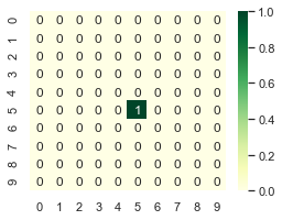
- Create initial configuration: We can use a vacant list to create initial configuration where initially particle is at middle of the lattice.
def start(L):
    '''create a vacant list of list '''
    P =  [[0 for i in range(L)]for j in range(L)]

    '''put particle at center'''
    P[int(L/2)][int(L/2)] = 1

    return P
P =start(L)
P
[[0, 0, 0, 0, 0, 0, 0, 0, 0, 0],
 [0, 0, 0, 0, 0, 0, 0, 0, 0, 0],
 [0, 0, 0, 0, 0, 0, 0, 0, 0, 0],
 [0, 0, 0, 0, 0, 0, 0, 0, 0, 0],
 [0, 0, 0, 0, 0, 0, 0, 0, 0, 0],
 [0, 0, 0, 0, 0, 1, 0, 0, 0, 0],
 [0, 0, 0, 0, 0, 0, 0, 0, 0, 0],
 [0, 0, 0, 0, 0, 0, 0, 0, 0, 0],
 [0, 0, 0, 0, 0, 0, 0, 0, 0, 0],
 [0, 0, 0, 0, 0, 0, 0, 0, 0, 0]]
- Make a plot of the lattice.
plt.figure(figsize = [4,3])
sns.heatmap(P,annot=True,cmap='YlGn')
<matplotlib.axes._subplots.AxesSubplot at 0x7fc8fdae7790>
- Create a function to diffuse a particle:
\( P[i,j] = P[i+1,j] + P[i-1,j] + P[i,j+1] + P[i,j-1] \)
def diffuse_primitive(P,L):

    '''create vacant list of list'''
    PP =  [[0 for i in range(L)]for j in range(L)]

    for i in range(L):
          for j in range(L):
                '''diffuse one step'''
                PP[i][j] = P[i+1][j] + P[i-1][j] + P[i][j+1] + P[i][j-1]

    '''normalize'''
    PP = PP/np.sum(PP)

    return PP
L =10
P =start(L)
-
Set boundary conditons
-
Lower limit
P[0-1,j] = P[L,j]
P[I,0-1] = P[i,L]
- Upper limit
P[L+1,j] = P[o,j]
P[i,L+1] = P[i,0]
def diffuse(P,L):

    '''create vacant list of list'''
    PP =  [[0 for i in range(L)]for j in range(L)]

    '''diffuse 1-step over supplied configuration'''
    for i in range(L):
          for j in range(L):

            '''set boundary condition at bottom and left'''
            ni =0; nj =0
            if i==0:ni = L
            if j==0:nj = L

            '''add modulo to control boundary at top and right'''
            PP[i][j] = P[(i+1)%L][j] + P[(i-1) + ni][j]\
            + P[i][(j+1)%L] + P[i][(j-1)+nj]

    '''normalize'''
    PP = PP/np.sum(PP)

    return PP
L =10
P =start(L)
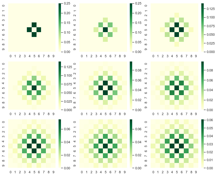
plt.figure(figsize = [12,10])
plt.subplot(3,3,1)
P = diffuse(P,L)
sns.heatmap(P,annot=False,cmap='YlGn')
plt.subplot(3,3,2)
P = diffuse(P,L)
sns.heatmap(P,annot=False,cmap='YlGn')
plt.subplot(3,3,3)
P = diffuse(P,L)
sns.heatmap(P,annot=False,cmap='YlGn')
plt.subplot(3,3,4)
P = diffuse(P,L)
sns.heatmap(P,annot=False,cmap='YlGn')
plt.subplot(3,3,5)
P = diffuse(P,L)
sns.heatmap(P,annot=False,cmap='YlGn')
plt.subplot(3,3,6)
P = diffuse(P,L)
sns.heatmap(P,annot=False,cmap='YlGn')
plt.subplot(3,3,7)
P = diffuse(P,L)
sns.heatmap(P,annot=False,cmap='YlGn')
plt.subplot(3,3,8)
P = diffuse(P,L)
sns.heatmap(P,annot=False,cmap='YlGn')
plt.subplot(3,3,9)
P = diffuse(P,L)
sns.heatmap(P,annot=False,cmap='YlGn')
plt.show()
- Run the diffusion step with desire no of running steps
def run_diffuse(P,nrun,L):

    run = 0

    '''diffuse N times'''
    while run < nrun:
        P = diffuse(P,L)
        run = run+1
    return P
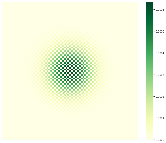
We can make a plot of arbitraty diffusion step by selecting irun in function runner.
'''set parameters'''
L = 100 ; nrun = 1000 ; P = start(L)

'''run diffusion'''
P = run_diffuse(P,nrun,L)
plt.figure(figsize = [12,10])
sns.heatmap(P,annot=False,cmap='YlGn')
plt.axis(False)
plt.show()
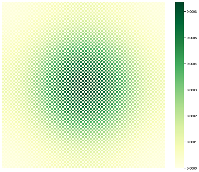
Much Finner
L = 200
nrun = 1000
P = start(L)

'''run diffusion'''
P = run_diffuse(P,nrun,L)
plt.figure(figsize = [12,10])
sns.heatmap(P,annot=False,cmap='YlGn')
plt.axis(False)
plt.show()